Function Plot
[1]:
from smpl import plot
import numpy as np
without uncertainties
\(\dot x = 1- \exp(- x^2)\)
Fixed point \(x = 0\) and
\(\ddot x = -2x \exp(-x^2) \implies \ddot x(x = 0)=0\)
only metastable for \(x\lt0\)
[2]:
plot.function( lambda x : 1- np.exp(-x**2), xaxis="$x$", yaxis="$\\dot x$",xmin=-10, xmax=10 )

\(\dot x = \ln x\)
Fixed point \(x = 1\)
\[\ddot x = \frac{1}{x} \implies \ddot x(x=1) = 1 > 0\]
\(\implies\) unstable
[3]:
plot.function( lambda x : np.log(x), xaxis="$x$", yaxis="$\\dot x$",xmin=0.1, xmax=5 )

\(\dot x = -\tan x\)
Fixed points for \(x=0\) or \(x=\pm n\pi\) with \(n\in \mathbb{N}\)
\[\ddot x = -\frac{1}{\cos^2(x)}\]
\[\ddot x(x=0) = -1 \lt 0\]
\[\ddot x(x=n \pi) = -1 \lt 0\]
\(\implies\) stable
[4]:
plot.function( lambda x : -np.tan(x), xaxis="$x$", yaxis="$\\dot x$",xmin=0.1, xmax=5,steps=100 )

with uncertainties
[5]:
import uncertainties as unc
a = unc.ufloat(1,0.1)
[6]:
plot.function(lambda x : 1- a*np.exp(-x**2), xaxis="$x$", yaxis="$\\dot x$",xmin=-1, xmax=1,sigmas=1 )

Complex
[7]:
from smpl.stat import fft
y = np.sin(np.arange(256))
print(len(fft(y)))
plot.data(*fft(y),label="FFT",fmt="-")
2
[7]:
(None, None)
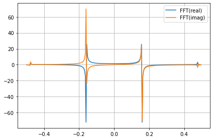
[8]:
from smpl.stat import fft
plot.data(*fft(np.sin(np.arange(256))),*fft(np.sin(1/np.pi*np.arange(100))),label="FFT",fmt="-")
[8]:
[(None, None), (None, None)]

[ ]: