Function Plot

[1]:

import numpy as np

import smpl
from smpl import plot

smpl.__version__

[1]:

'1.4.2'

without uncertainties

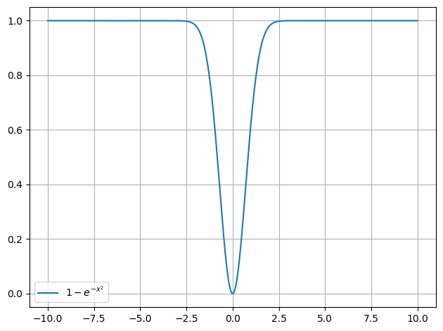
\(\dot x = 1- \exp(- x^2)\)

Fixed point \(x = 0\) and

\(\ddot x = -2x \exp(-x^2) \implies \ddot x(x = 0)=0\)

only metastable for \(x\lt0\)

[2]:

plot.function(
    lambda x: 1 - np.exp(-(x**2)), xaxis="$x$", yaxis="$\\dot x$", xmin=-10, xmax=10
)

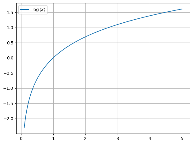
../../../_images/example_plot_functions_funcs_4_0.png

\(\dot x = \ln x\)

Fixed point \(x = 1\)

\[\ddot x = \frac{1}{x} \implies \ddot x(x=1) = 1 > 0\]

\(\implies\) unstable

[3]:

plot.function(lambda x: np.log(x), xaxis="$x$", yaxis="$\\dot x$", xmin=0.1, xmax=5)

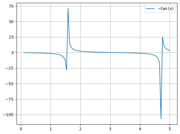
../../../_images/example_plot_functions_funcs_6_0.png

\(\dot x = -\tan x\)

Fixed points for \(x=0\) or \(x=\pm n\pi\) with \(n\in \mathbb{N}\)

\[\ddot x = -\frac{1}{\cos^2(x)}\]

\[\ddot x(x=0) = -1 \lt 0\]

\[\ddot x(x=n \pi) = -1 \lt 0\]

\(\implies\) stable

[4]:

plot.function(
    lambda x: -np.tan(x), xaxis="$x$", yaxis="$\\dot x$", xmin=0.1, xmax=5, steps=100
)

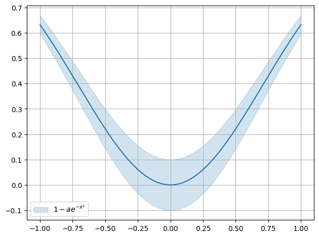
../../../_images/example_plot_functions_funcs_8_0.png

with uncertainties

[5]:

import uncertainties as unc

a = unc.ufloat(1, 0.1)

[6]:

plot.function(
    lambda x: 1 - a * np.exp(-(x**2)),
    xaxis="$x$",
    yaxis="$\\dot x$",
    xmin=-1,
    xmax=1,
    sigmas=1,
)

../../../_images/example_plot_functions_funcs_11_0.png

Complex

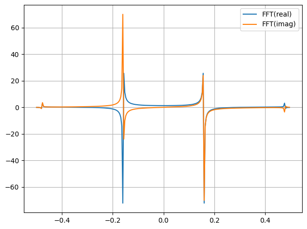
[7]:

from smpl.stat import fft

y = np.sin(np.arange(256))
print(len(fft(y)))
plot.data(*fft(y), label="FFT", fmt="-")

[7]:

(None, None)

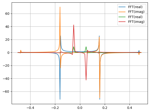
../../../_images/example_plot_functions_funcs_13_2.png

[8]:

from smpl.stat import fft

plot.data(
    *fft(np.sin(np.arange(256))),
    *fft(np.sin(1 / np.pi * np.arange(100))),
    label="FFT",
    fmt="-",
)

[8]:

[(None, None), (None, None)]

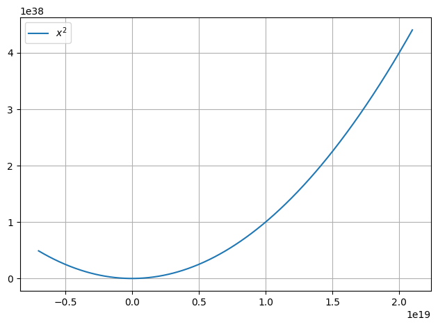
../../../_images/example_plot_functions_funcs_14_1.png

without xmin and xmax

xmin and xmax will have to be guessed

[9]:

from smpl import plot

plot.function(
    lambda x: x**2,
)

/home/docs/checkouts/readthedocs.org/user_builds/smpl/envs/v1.4.2/lib/python3.12/site-packages/numpy/_core/function_base.py:162: RuntimeWarning: overflow encountered in multiply
  y *= step
/tmp/ipykernel_1720/1358134803.py:4: RuntimeWarning: overflow encountered in square
  lambda x: x**2,

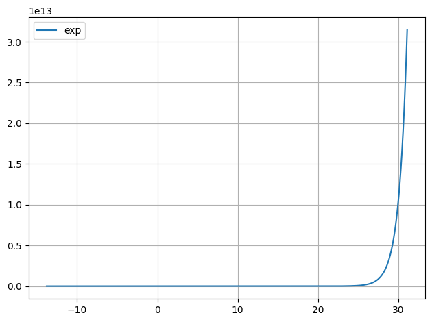
../../../_images/example_plot_functions_funcs_16_1.png

[10]:

import numpy as np

from smpl import plot

def f(x):
    return np.exp(x)

plot.function(f, label="exp")

/tmp/ipykernel_1720/682357243.py:7: RuntimeWarning: overflow encountered in exp
  return np.exp(x)

../../../_images/example_plot_functions_funcs_17_1.png

[11]:

from smpl import functions as f
from smpl import plot


def gauss(x):
    """Gauss"""
    return f.gauss(x, 0, 1, 3, 0)


plot.function(gauss)

/home/docs/checkouts/readthedocs.org/user_builds/smpl/envs/v1.4.2/lib/python3.12/site-packages/smpl/functions.py:76: RuntimeWarning: overflow encountered in square
  return a * unp.exp(-((x - x_0) ** 2) / 2 / d**2) + y

../../../_images/example_plot_functions_funcs_18_1.png

[12]:

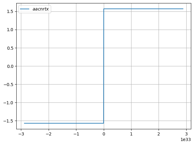
def gauss(x):
    return np.arctan(x)


plot.function(gauss)

../../../_images/example_plot_functions_funcs_19_0.png

[13]:

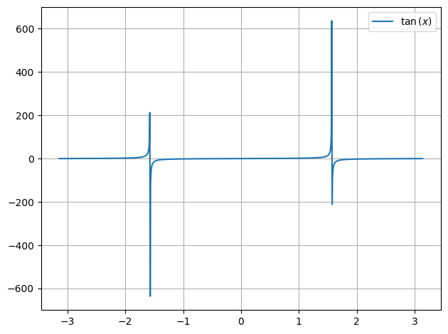
def gauss(x):
    return np.tan(x)


plot.function(gauss)

../../../_images/example_plot_functions_funcs_20_0.png

[14]:

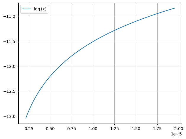
def gauss(x):
    return np.log(x)


plot.function(gauss)

/tmp/ipykernel_1720/871555150.py:2: RuntimeWarning: invalid value encountered in log
  return np.log(x)

../../../_images/example_plot_functions_funcs_21_1.png

[15]:

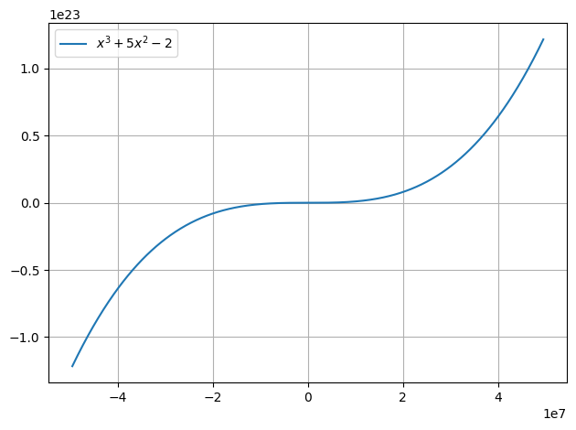
def gauss(x):
    return x**3 + 5 * x**2 - 2


plot.function(gauss)

/tmp/ipykernel_1720/3023670006.py:2: RuntimeWarning: overflow encountered in power
  return x**3 + 5 * x**2 - 2
/tmp/ipykernel_1720/3023670006.py:2: RuntimeWarning: overflow encountered in square
  return x**3 + 5 * x**2 - 2
/tmp/ipykernel_1720/3023670006.py:2: RuntimeWarning: invalid value encountered in add
  return x**3 + 5 * x**2 - 2
/tmp/ipykernel_1720/3023670006.py:2: RuntimeWarning: overflow encountered in multiply
  return x**3 + 5 * x**2 - 2

../../../_images/example_plot_functions_funcs_22_1.png

[16]:

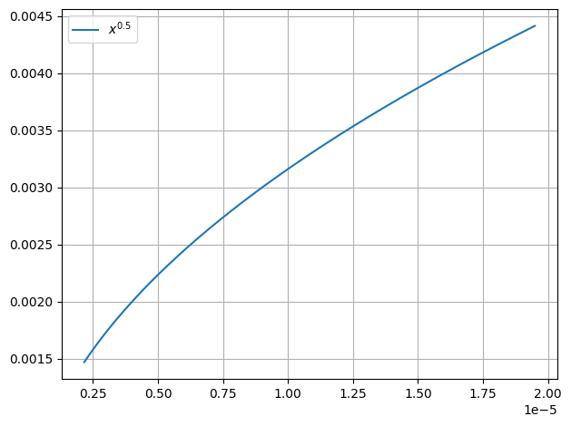
def gauss(x):
    return x**0.5


plot.function(gauss)

/tmp/ipykernel_1720/2383082664.py:2: RuntimeWarning: invalid value encountered in sqrt
  return x**0.5

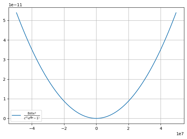
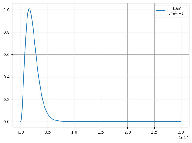
../../../_images/example_plot_functions_funcs_23_1.png

Guessing the interesting regions of a function can’t always be correct/satisfactory, especially in numerical unstable regions:

[17]:

c = 299792458  # m/s
h = 4.13566769692 * 10**-15  # eVs
kb = 8.617333262 * 10**-5  # eV/K
T = 273


def Strahlungsgesetz(x):
    return 8 * np.pi / c**3 * h * x**3 / (np.exp((h * x) / (kb * T)) - 1)


plot.function(Strahlungsgesetz, xaxis="$x$", yaxis="$\\dot x$")

/tmp/ipykernel_1720/1614935106.py:8: RuntimeWarning: overflow encountered in power
  return 8 * np.pi / c**3 * h * x**3 / (np.exp((h * x) / (kb * T)) - 1)
/tmp/ipykernel_1720/1614935106.py:8: RuntimeWarning: overflow encountered in exp
  return 8 * np.pi / c**3 * h * x**3 / (np.exp((h * x) / (kb * T)) - 1)
/tmp/ipykernel_1720/1614935106.py:8: RuntimeWarning: invalid value encountered in divide
  return 8 * np.pi / c**3 * h * x**3 / (np.exp((h * x) / (kb * T)) - 1)
/tmp/ipykernel_1720/1614935106.py:8: RuntimeWarning: divide by zero encountered in divide
  return 8 * np.pi / c**3 * h * x**3 / (np.exp((h * x) / (kb * T)) - 1)
/home/docs/checkouts/readthedocs.org/user_builds/smpl/envs/v1.4.2/lib/python3.12/site-packages/scipy/optimize/_optimize.py:851: RuntimeWarning: invalid value encountered in subtract
  np.max(np.abs(fsim[0] - fsim[1:])) <= fatol):
/home/docs/checkouts/readthedocs.org/user_builds/smpl/envs/v1.4.2/lib/python3.12/site-packages/smpl/stat.py:160: RuntimeWarning: invalid value encountered in multiply
  val += weights[k] * func(x0 + (k - ho) * dx, *args)

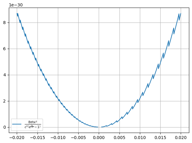
../../../_images/example_plot_functions_funcs_25_1.png

[18]:

plot.function(
    Strahlungsgesetz, xaxis="$x$", yaxis="$\\dot x$", xmin=1e-7 - 2e-2, xmax=1e-7 + 2e-2
)

/tmp/ipykernel_1720/1614935106.py:8: RuntimeWarning: divide by zero encountered in divide
  return 8 * np.pi / c**3 * h * x**3 / (np.exp((h * x) / (kb * T)) - 1)

../../../_images/example_plot_functions_funcs_26_1.png

[19]:

plot.function(Strahlungsgesetz, xaxis="$x$", yaxis="$\\dot x$", xmin=1, xmax=0.3e15)

../../../_images/example_plot_functions_funcs_27_0.png

[ ]: